Policy: Epsilon First

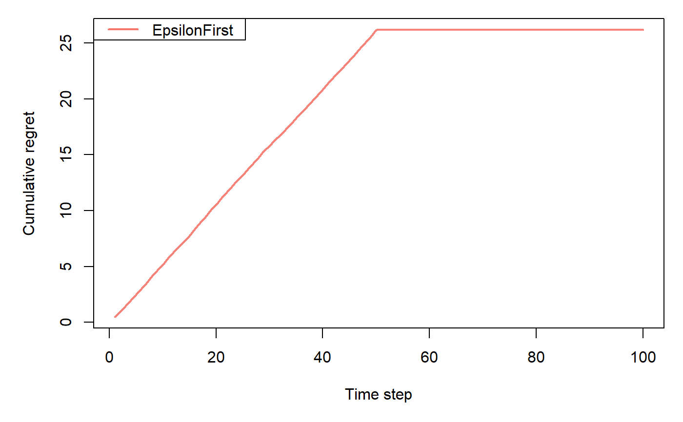
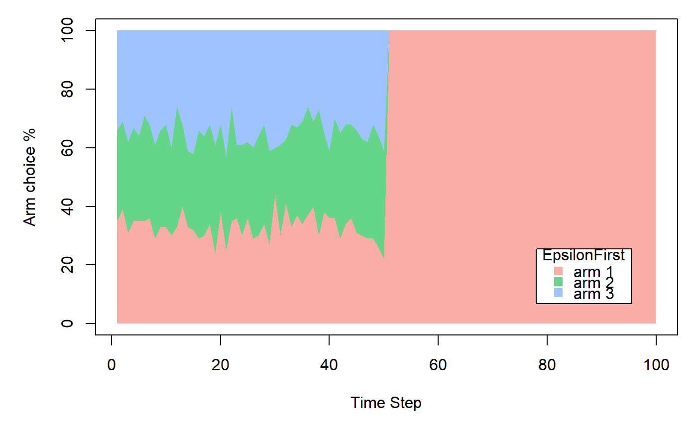
EpsilonFirstPolicy implements a "naive" policy where a pure exploration phase is followed by a pure exploitation phase.

Details

Exploration happens within the first epsilon * N time steps. During this time, at each time step t, EpsilonFirstPolicy selects an arm at random.

Exploitation happens in the following (1-epsilon) * N steps, selecting the best arm up until epsilon * N for either the remaining N trials or horizon T.

In case of a tie in the exploitation phase, EpsilonFirstPolicy randomly selects and arm.

Usage

policy <- EpsilonFirstPolicy(epsilon = 0.1, N = 1000, time_steps = NULL)

Arguments

epsilon

numeric; value in the closed interval (0,1] that sets the number of time steps to explore through epsilon * N.

N

integer; positive integer which sets the number of time steps to explore through epsilon * N.

time_steps

integer; positive integer which sets the number of time steps to explore - can be used instead of epsilon and N.

Methods

new(epsilon = 0.1, N = 1000, time_steps = NULL)

Generates a new EpsilonFirstPolicy object. Arguments are defined in the Argument section above.

set_parameters()

each policy needs to assign the parameters it wants to keep track of to list self$theta_to_arms that has to be defined in set_parameters()'s body. The parameters defined here can later be accessed by arm index in the following way: theta[[index_of_arm]]$parameter_name

get_action(context)

here, a policy decides which arm to choose, based on the current values of its parameters and, potentially, the current context.

set_reward(reward, context)

in set_reward(reward, context), a policy updates its parameter values based on the reward received, and, potentially, the current context.

References

Gittins, J., Glazebrook, K., & Weber, R. (2011). Multi-armed bandit allocation indices. John Wiley & Sons. (Original work published 1989)

Sutton, R. S. (1996). Generalization in reinforcement learning: Successful examples using sparse coarse coding. In Advances in neural information processing systems (pp. 1038-1044).

Strehl, A., & Littman, M. (2004). Exploration via model based interval estimation. In International Conference on Machine Learning, number Icml.

See also

Core contextual classes: Bandit, Policy, Simulator, Agent, History, Plot

Bandit subclass examples: BasicBernoulliBandit, ContextualLogitBandit, OfflineReplayEvaluatorBandit

Policy subclass examples: EpsilonGreedyPolicy, ContextualLinTSPolicy

Examples

horizon            <- 100L
simulations        <- 100L
weights            <- c(0.9, 0.1, 0.1)

policy             <- EpsilonFirstPolicy$new(time_steps = 50)
bandit             <- BasicBernoulliBandit$new(weights = weights)
agent              <- Agent$new(policy, bandit)

history            <- Simulator$new(agent, horizon, simulations, do_parallel = FALSE)$run()
#> Simulation horizon: 100
#> Number of simulations: 100
#> Number of batches: 1
#> Starting main loop.
#> Finished main loop.
#> Completed simulation in 0:00:01.161
#> Computing statistics.

plot(history, type = "cumulative")
plot(history, type = "arms")