The Inverse Gamma Distribution — invgamma • contextual

Density, distribution function, quantile function and random generation for the inverse gamma distribution.

dinvgamma(x, shape, rate = 1, scale = 1/rate, log = FALSE)

pinvgamma(q, shape, rate = 1, scale = 1/rate, lower.tail = TRUE, log.p = FALSE)

qinvgamma(p, shape, rate = 1, scale = 1/rate, lower.tail = TRUE, log.p = FALSE)

rinvgamma(n, shape, rate = 1, scale = 1/rate)

Arguments

x, q	vector of quantiles.
shape	inverse gamma shape parameter
rate	inverse gamma rate parameter
scale	alternative to rate; scale = 1/rate
log, log.p	logical; if TRUE, probabilities p are given as log(p).
lower.tail	logical; if TRUE (default), probabilities are P(X <= x) otherwise, P(X > x).
p	vector of probabilities.
n	number of observations. If length(n) > 1, the length is taken to be the number required.

Details

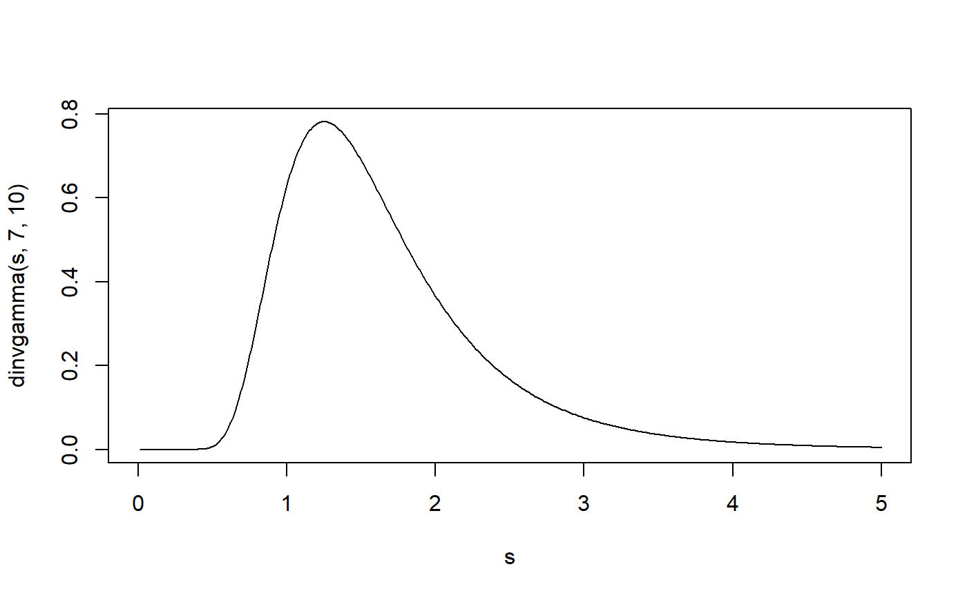
The inverse gamma distribution with parameters shape and rate has density f(x) = rate^shape/Gamma(shape) x^(-1-shape) e^(-rate/x) it is the inverse of the standard gamma parameterization in R.

The functions (d/p/q/r)invgamma simply wrap those of the standard (d/p/q/r)gamma R implementation, so look at, say, dgamma for details.

Examples


s <- seq(0, 5, .01)
plot(s, dinvgamma(s, 7, 10), type = 'l')

f <- function(x) dinvgamma(x, 7, 10)
q <- 2
integrate(f, 0, q)
#> 0.7621835 with absolute error < 7.3e-05
(p <- pinvgamma(q, 7, 10))
#> [1] 0.7621835
qinvgamma(p, 7, 10) # = q
#> [1] 2
mean(rinvgamma(1e5, 7, 10) <= q)
#> [1] 0.76049